Motivation
The year is 2019. It's a chilly October morning. You wake up and head to your kitchen.
Suddenly, there's a knock on your door. What could that be? You open the door and, to your
surprise, there are 150 delivered floor lamps on your front porch. You check your bank account statement and yep,
you paid for them. What? How? Who?
Your voice assistant, Alexa, can order items through Amazon. I, a malicious hacker, recorded a snippet of
your voice. I used that small snippet to recreate you saying "Hey Alexa, order 150 floor lamps!". I embedded
it on a site you regularly visit and Alexa, ever diligent, heard it play through your computer speakers and
ordered you the floor lamps "you" wanted. It would make sense that this
system will ultimately include some sort of biometric protection to ensure that your voice
(i.e., the voice that ordered 150 floor lamps) is indeed your voice and not, say, some
text-to-speech neural model that can emulate your voice. Well, at least we ought to hope,
unless of course you're in the market for 150 floor lamps.
This is a silly example. How about a more pressing one? Your bank thought that it was too easy
to hack passwords. It's really hard to hack the human voice. It sets up biometric security on your bank
account so all you have to do is say a random phrase into a microphone and then you get full access to your
account if the voice it just listened to matches the profile of a voice it knows is yours. I, still a malicious
hacker, records you talking. I use some machine learning and have a program that can emulate
your voice perfectly. I play it to your bank's log in screen and I wire myself your entire savings.
I blow the money on floor lamps and have them all shipped to you. Now, you have no money, and I have a much
more realistic example of why the work I'm about to describe is important.
Protecting voice activated systems against these sorts of attacks
— especially as developers create more and more features that are integrated with your bank
— is super important. In machine-learning-startup-valley, generative
adversarial networks (GANs for short) are common talk. Everybody knows about them. With AWS
catering to the whims of every machine learning engineer out there, it's trivial (okay, maybe
not trivial, but no more than a weeks' amount of work) to get one up and running on a cluster
of performant servers. With a small snippet of your voice, these networks can be impersonating
you within hours of training. Your living room just got a lot brighter.
So what can we do?
What we can do
For several years, there's been a concerted effort within the research community to address
the growing threats posed by these sorts of malicious attacks. A notable conference,
Interspeech, has been hosting a challenge since 2015 focusing on voice spoofing. It's called
ASVspoof, and the latest addition to it, ASVspoof 2019, just wrapped up in Gratz, Austria.
The competition has grown and now sees incredibly diverse attempts at solving this problem.
From the frontend to the backend, each leading entrant has pushed the understanding of the
problem forward.
This semester, I'm taking a course in machine learning for signal processing (MLSP for short).
Its focus is to better understand machine learning within the context of traditional signal
processing and use recent advances in machine learning to create more robust methods of
understanding data from signals. We have a semester long project to study some application
of machine learning to signal processing.
My team and I are aiming our project to better understand why some types of features and some
types of models are particularly good at distinguishing spoofed speech from genuine speech.
Technical context
To understand our approach, let's take a quick dive into some technicalities. Here's the motivating
problem: we need to represent audio on a computer. There are probably an infinite number of ways
we could do this. The problem is really open-ended. Let's look at a way that we're all relatively
familiar with.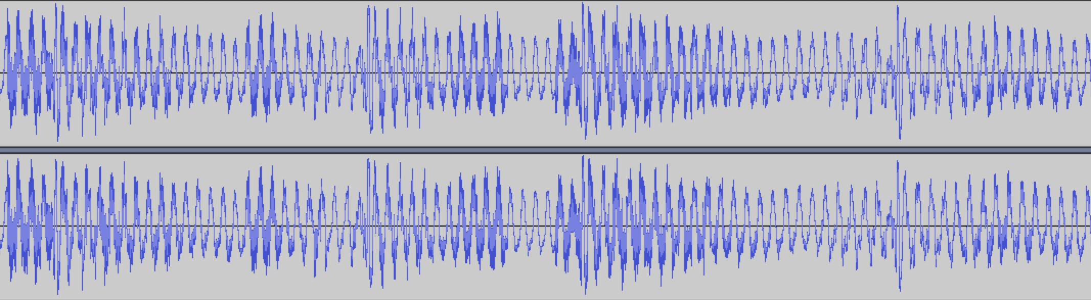 A time waveform, an intuitive way of representing audio.
The image above is a representation of audio called a waveform. It represents the pressure exerted
by a sound wave on a microphone as a function of time. Our ear drums work similarly. As sound
travels to us, our ear drums vibrate according to the pressure. This variant pressure is converted
into electrical pulses that are further processed.
This is a super useful way of representing sound. There are other ways though! A very common trend
is to represent audio according to the frequency that makes up a particular segment of it. We use a
variety of representations to explore these frequencies. Let's look at two.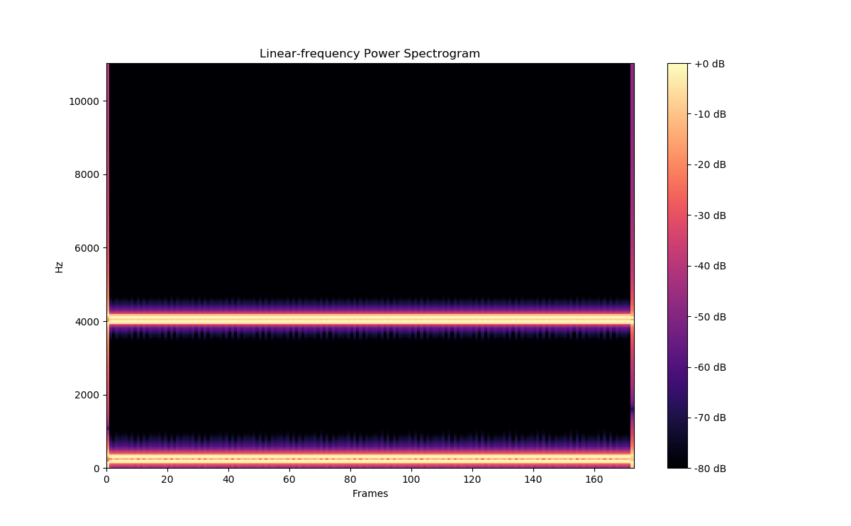 A spectrogram, a standard way of representing the frequencies that comprise signals.
The Fourier transform can take an input signal and return the frequencies that comprise the signal.
Imagine giving a Fourier Transform a guitar chord, it would give you back the notes in the chord.
This is an amazing tool and it's used everywhere. Here's the equation for getting the Fourier Transform
, \(X(e^{j\omega})\), of an input, \(x(t)\):
\[ X(e^{j\omega}) = \int_{\infty}^{+\infty} x(t) e^{-j \omega t} dt. \]
This looks super complicated, but, after struggling under the toil of dozens of hours of manual
Fourier Transform computations, I promise it doesn't get any easier! It's still super complicated
and magical.
The spectrogram above represents a picture of the Fourier Transform of a signal at different time points.
We take a signal, section it off into small chunks (for speech signals, the chunks are around 20ms), then
we compute the Fourier Transform of those chunks and shove them into a picture. The horizontal axis is time.
The vertical axis is frequency. The color represents the magnitude of the frequency component. So, from the
spectrogram above, we can see that the input signal was made of four frequencies, some that are around
250 Hz and some that are up around 4,000 Hz. You may only see two horizontal bars. If you zoom in close
enough, you should see some faint distinction in the middles of the two bars. That's how we know there are four
frequencies in the signal.
The important parts of speech signals are always on the lower end of the spectrum (50 - 300 Hz). If we look
at the spectrogram above, we can see there's a lot of wasted space and not that much separation
between those lower frequency components. If we want to do something like speech processing, we're going to
need much better resolution at those lower frequencies. Cue the mel-spectrogram!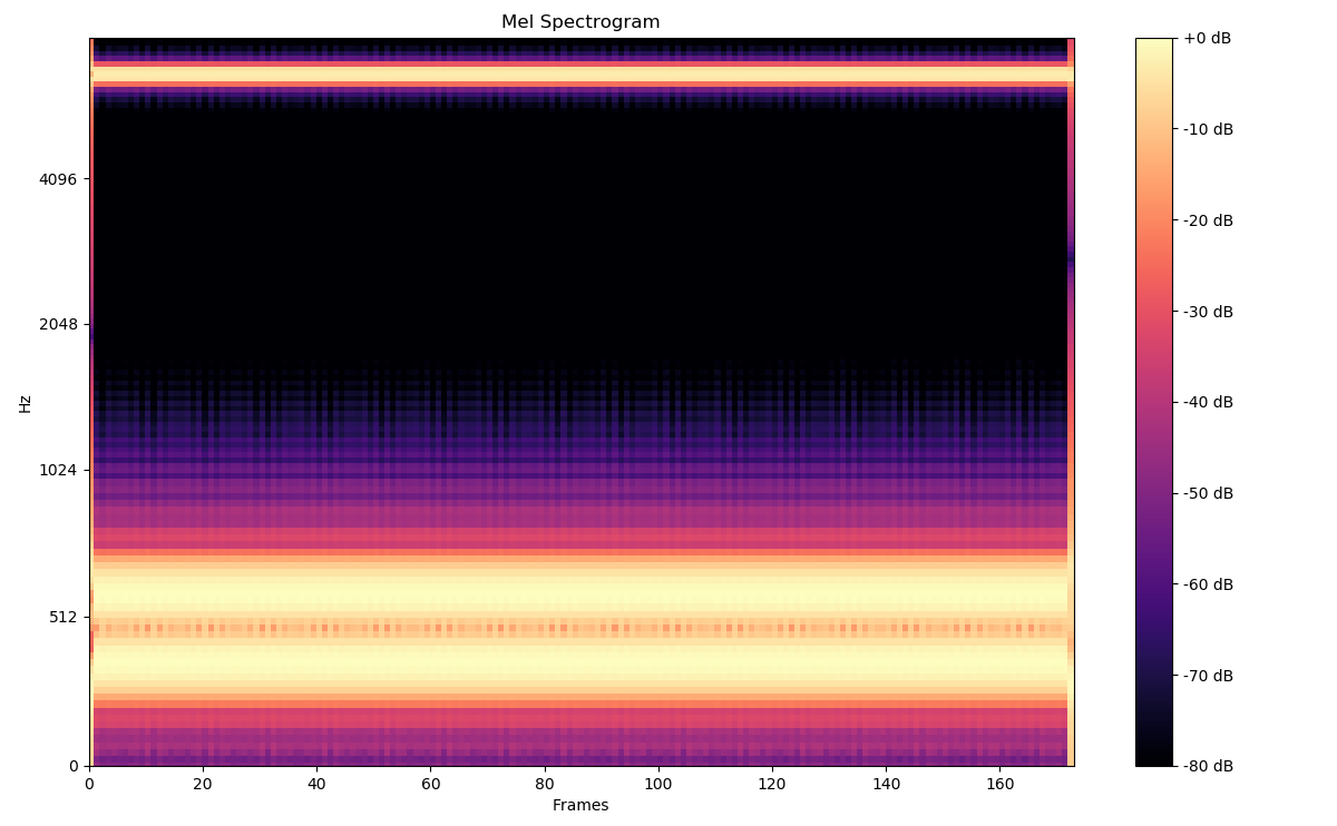 A mel-spectrogram, a standard way of representing speech-like signals.
Some initial reactions: this looks a lot like the other spectrogram. But look at the vertical axis' scale!
Instead of being linear (like the other spectrogram), this one is logarithmically scaled. That is, the first
tick is at 512, the next is at 1024, the next is at 2048, etc. It doubles every time. And that has real
consequences! We are now able to distinguish between those lower frequencies really well. Please note,
this is essentially the same signal as the one in the previous spectrogram. Whereas it was difficult to make
out the two separate frequencies on the lower end of the spectrum, now it's super easy to see that there are
indeed two frequencies there.
We aren't able to
distinguish between the higher frequencies at all, though. That's fine! Remember, the important parts of
speech are at lower frequencies. This is a very important tool in all speech-related signal processing.
There are other types of transforms like these. A notable one is called the Constant-Q transform. It's
great at representing music. We won't dive into those too much here but it suffices to say they are
very similar to the mel-frequency scaled transforms.
Some trends
We are fascinated by a central theme in many of the leading submissions to the competition:
constant-Q cepstral coefficients (CQCC) outperforming mel-frequency cepstral coefficients (MFCC).
These coefficients are different from the spectrograms shown above but maintain some similar poetic
properties vis a vis their resolutions at low versus high frequencies.
There are also some other interesting trends relating to CQCCs. One entrant proposed an inverted
frequency scale to be used in the calculation of CQCCs.
The inverted frequency scale in these features refers to modifying standard MFCCs and CQCCs to have very
fine resolution at high frequencies and very low resolution at low frequencies. If you look at the
mel-spectrogram above, you can see that it has fine resolution at the low frequencies and awful resolution
at the higher frequencies. It's really surprising that inverting that scale (i.e., lots of resolution at
high frequencies and bad resolution at the low frequencies) would lead to better performance. We have a couple thoughts about
why this sort of feature works particularly well for recognizing spoofed speech.
When things are recorded and played back via a speaker, the processing that takes place during recording,
saving, and playback will leave hardly-noticeable high frequency content in the artifact that is then picked
up by Alexa or Siri or whomever. When systems can see clearer pictures of what's going on at those high frequencies,
they are more adept at recognizing when they're listening to pre-recorded speech.
Our plan
We want to test this hypothesis and several others. To do so, we're going to create two very standard models:
a Gaussian mixture model (GMM) and a support vector machine (SVM). We'll feed them both all kinds of features
related to MFCCs and CQCCs.
After the first round of experiments, we'll be able to tell which feature-model pair performs best ("best" here
refers to ASVspoof 2019's EER and t-DCF metrics). Next, we'll do some digging and come up with reasons why these
pairs are performing well. We'll test those hypotheses with a second round of experiments.
After the second round, we'll have a pretty good idea of what works and, most importantly, why it works well.
We'll write all of this up into a report and see what people think.
I'm working on this project with Mark Lindsey.